Feature detection and randomness
What could it possibly have to do with my life?
Feature detection
descriptors
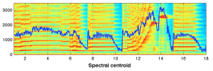
- Spectral
- BarkBands, MelBands, ERBBands, MFCC, GFCC, LPC, HFC, Spectral Contrast, Inharmonicity, and Dissonance, …
- Time-domain
- EffectiveDuration, ECR, Loundness, …
- Tonal
- PitchSalienceFunction, PitchYinFFT, HPCP, TuningFrequency, Key, ChordsDetection, …
- Rhythm
- BestTrackerDegara, BeatTrackerMultiFeature, BPMHistogramDescriptors, NoveltyCurve, OnsetDescription, OnsetDetection, Onsets, …
- SFX
- LogAttackTime, MaxToTotal, MinToTotal, TCToTotal, …
- High-level
- Danceability, DynamicComplexity, FadeDetection, SBic, …
-from X. Serra (2014) “Audio Signal Processing for Music Applications”
- low level vs. high level
- single events vs. groups of events
- combinations of descriptors
- order of events (markov chains)
Humans are very good at pattern recognition. Is it a survival mechanism? People who listen to music are very good at analysis. Compared to the abilities of an average child, computer music information retrieval has not yet reached the computational ability of a worm: https://reactivemusic.net/?p=17744
Pattern recognition
(in computer science)
Music information retrieval
High-level
Low-level
(These demonstrations will be done in Ubuntu Linux 14.04.1)
1. Separating and removing musical tones from speech
1a. Harmonic plus residual model (HPR) in sms-tools (speech-female 150-200 Hz. , and sax phrase)
1b. Do the same thing with transformation model
What about pitch salience and chroma?
2. descriptors
(use workspace/A9)
import soundAnalysis as SA
Here is the list of descriptors that are donwloaded:
Index — Descriptor
0 — lowlevel.spectral_centroid.mean
1 — lowlevel.dissonance.mean
2 — lowlevel.hfc.mean
3 — sfx.logattacktime.mean
4 — sfx.inharmonicity.mean
5 — lowlevel.spectral_contrast.mean.0
6 — lowlevel.spectral_contrast.mean.1
7 — lowlevel.spectral_contrast.mean.2
8 — lowlevel.spectral_contrast.mean.3
9 — lowlevel.spectral_contrast.mean.4
10 — lowlevel.spectral_contrast.mean.5
11 — lowlevel.mfcc.mean.0
12 — lowlevel.mfcc.mean.1
13 — lowlevel.mfcc.mean.2
14 — lowlevel.mfcc.mean.3
15 — lowlevel.mfcc.mean.4
16 — lowlevel.mfcc.mean.5
2a. euclidian distance
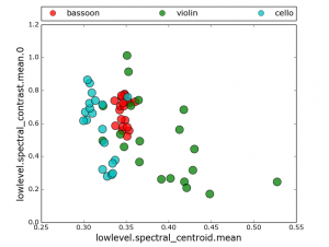
What happens when you look at multiple descriptors
In [22]: SA.descriptorPairScatterPlot( ‘tmp’, descInput=(0,5))

2b. k- means clustering
What descriptors best classify sounds into instrument groups?
SA.clusterSounds(‘tmp’, nCluster = 3, descInput=[0,2,9])
In [21]: SA.clusterSounds(‘tmp’, nCluster = 3, descInput=[0,2,9])
(Cluster: 0) Using majority voting as a criterion this cluster belongs to class: violin
Number of sounds in this cluster are: 15
sound-id, sound-class, classification decision
[[‘61926’ ‘violin’ ‘1’]
[‘61925’ ‘violin’ ‘1’]
[‘153607’ ‘violin’ ‘1’]
[‘153629’ ‘violin’ ‘1’]
[‘153609’ ‘violin’ ‘1’]
[‘153608’ ‘violin’ ‘1’]
[‘153628’ ‘violin’ ‘1’]
[‘153603’ ‘violin’ ‘1’]
[‘153602’ ‘violin’ ‘1’]
[‘153601’ ‘violin’ ‘1’]
[‘153600’ ‘violin’ ‘1’]
[‘153610’ ‘violin’ ‘1’]
[‘153606’ ‘violin’ ‘1’]
[‘153605’ ‘violin’ ‘1’]
[‘153604’ ‘violin’ ‘1’]]
(Cluster: 1) Using majority voting as a criterion this cluster belongs to class: bassoon
Number of sounds in this cluster are: 22
sound-id, sound-class, classification decision
[[‘154336’ ‘bassoon’ ‘1’]
[‘154337’ ‘bassoon’ ‘1’]
[‘154335’ ‘bassoon’ ‘1’]
[‘154352’ ‘bassoon’ ‘1’]
[‘154344’ ‘bassoon’ ‘1’]
[‘154338’ ‘bassoon’ ‘1’]
[‘154339’ ‘bassoon’ ‘1’]
[‘154343’ ‘bassoon’ ‘1’]
[‘154342’ ‘bassoon’ ‘1’]
[‘154341’ ‘bassoon’ ‘1’]
[‘154340’ ‘bassoon’ ‘1’]
[‘154347’ ‘bassoon’ ‘1’]
[‘154346’ ‘bassoon’ ‘1’]
[‘154345’ ‘bassoon’ ‘1’]
[‘154353’ ‘bassoon’ ‘1’]
[‘154350’ ‘bassoon’ ‘1’]
[‘154349’ ‘bassoon’ ‘1’]
[‘154348’ ‘bassoon’ ‘1’]
[‘154351’ ‘bassoon’ ‘1’]
[‘61927’ ‘violin’ ‘0’]
[‘61928’ ‘violin’ ‘0’]
[‘153769’ ‘cello’ ‘0’]]
(Cluster: 2) Using majority voting as a criterion this cluster belongs to class: cello
Number of sounds in this cluster are: 23
sound-id, sound-class, classification decision
[[‘154334’ ‘bassoon’ ‘0’]
[‘61929’ ‘violin’ ‘0’]
[‘61930’ ‘violin’ ‘0’]
[‘153626’ ‘violin’ ‘0’]
[‘42252’ ‘cello’ ‘1’]
[‘42250’ ‘cello’ ‘1’]
[‘42251’ ‘cello’ ‘1’]
[‘42256’ ‘cello’ ‘1’]
[‘42257’ ‘cello’ ‘1’]
[‘42254’ ‘cello’ ‘1’]
[‘42255’ ‘cello’ ‘1’]
[‘42249’ ‘cello’ ‘1’]
[‘42248’ ‘cello’ ‘1’]
[‘42247’ ‘cello’ ‘1’]
[‘42246’ ‘cello’ ‘1’]
[‘42239’ ‘cello’ ‘1’]
[‘42260’ ‘cello’ ‘1’]
[‘42241’ ‘cello’ ‘1’]
[‘42243’ ‘cello’ ‘1’]
[‘42242’ ‘cello’ ‘1’]
[‘42253’ ‘cello’ ‘1’]
[‘42244’ ‘cello’ ‘1’]
[‘42259’ ‘cello’ ‘1’]]
Out of 60 sounds, 7 sounds are incorrectly classified considering that one cluster should ideally contain sounds from only a single class
You obtain a classification (based on obtained clusters and majority voting) accuracy of 88.33 percentage
2c. KNN find nearest neighbors
Which neighborhood or group does a sound belong to?
(using bad male vocal)
SA.classifySoundkNN(“qs/175454/175454/175454_2042115-lq.json”, “tmp”,13, descInput = [0,5,10])
===
from workspace…
First test: Use sounds by querying “saxophone”, tag=”alto-sax”
https://www.freesound.org/people/clruwe/sounds/119248/
I am using the same descriptors [0,2,9] that worked well in previous section. with K=3. Tried various values of K with this analysis and it always came out matching ‘violin’ which I think is correct.
In [26]: SA.classifySoundkNN(“qs/saxophone/119248/119248_2104336-lq.json”, “tmp”, 33, descInput = [0,2,9])
This sample belongs to class: violin
Out[26]: ‘violin’
Second test: I am trying out the freesound “similar sound” feature. Using one of the bassoon sounds I clicked “similar sounds” and chose a sound that was not a bassoon – “Bad Singer” (male).
http://freesound.org/people/sergeeo/sounds/175454/
Running the previous descriptors returned a match for violin. So I tried various other descriptors, and was able to get it to match bassoon consistently by using: [0,5,10] which are lowlevel.spectral_centroid.mean, lowlevel.spectral_contrast.mean.0, and lowlevel.mfcc.mean.0.
I honestly don’t know the best strategy for choosing these descriptors and tried to go with ones that seemed the least esoteric. The value of K does not seem to make any difference in the classification.
Here is the output
In [42]: SA.classifySoundkNN(“qs/175454/175454/175454_2042115-lq.json”, “tmp”,13, descInput = [0,5,10])
This sample belongs to class: bassoon
Out[42]: ‘bassoon’
2d. JSON analysis data for “bad voice” example…
#: cd ~/sms-tools/workspace/A9/qs/175454/175454
# cat 175454_2042115-lq.json | python -mjson.tool
3. acousticbrainz
(typical analysis page…) https://reactivemusic.net/?p=17641
4. Echonest acoustic analysis
fingerprinting and human factors like danceability…
Randomness
continuum
random -> ordered (stochastic -> deterministic (for academics))
Does technology have a sound?
Can you add small bits of randomness?
- Can you detect randomness?
- How much repetition is enough?
Brain wiring diagram: https://reactivemusic.net/?p=17758
Christof Koch – check out this video at around 13:33 for about 2 minutes http://www.technologyreview.com/emtech/14/video/watch/christof-koch-hacking-the-soul/
With every technology, musicians figure out how to use it another way. Starting with stone tools, bow and arrow, and now computers.
Data science skills: https://reactivemusic.net/?p=17707
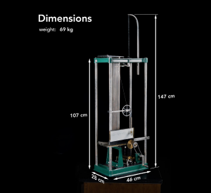
Car engine synthesizer
At the end of the class we revved the engine of a 2015 Golf TSI, connected to an engine sound simulator in Max, on Boylston street…
https://reactivemusic.net/?p=7643
