Interactive Web Audio synthesizer with visualization
Start watching around 2:00 to see the actual app.
Interactive Web Audio synthesizer with visualization
Start watching around 2:00 to see the actual app.
By Stephane Boucher at dsprelated.com
http://www.dsprelated.com/showarticle/584.php
Constructing a square wave with an infinite series
Facial recognition software for detecting emotions
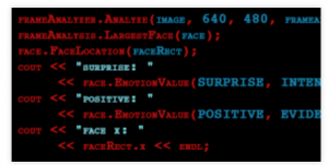
Emotient API: http://www.emotient.com/products#FACETSDK
“Intensely pleasurable responses to music correlate with activity in brain regions implicated in reward and emotion.”
By Anne J. Blood* and Robert J. Zatorre at Montreal Neurological Institute, McGill University (2001)
http://www.pnas.org/content/98/20/11818.full
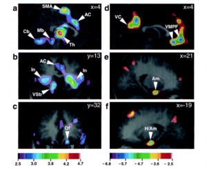
Also in “Berklee Today”, by Sarah Godcher: http://www.berklee.edu/bt/133/bb_neurology.html
“Results of the chills study also showed decreased activity in the areas of the brain that process danger and anxiety. “This says to me,” continued Blood, “that in order to experience this kind of euphoria, the part of the brain [that responds to danger] has to shut down. You can’t be euphoric and scared at the same time.”
The study also revealed that the brain processes consonant and dissonant sounds in very different ways. Dissonant sounds affected areas of the brain involving memory and anxiety, while consonant sounds stimulated areas involved in pleasant emotional responses. The results of Blood’s study may be validating through science what composers and performers of music have known for centuries.
Blood hastened to add that music’s ability to produce the chills is entirely subjective. All 10 of the subjects in the study selected classical music, but jazz and rock also can affect listeners just as powerfully, she said. Proof of this subjectivity can be found in a person’s response to music they did not select themselves. As each individual listened to a piece of music selected by one of the other nine subjects, “no one responded similarly to someone else’s music,” Blood said.
A significant aspect of Blood’s findings is that almost all of the brain’s response to music takes place at the subcortical level, that is in nerve centers below the cerebral cortex, which is the region of the brain where abstract thought occurs. Our brains process music, therefore, without really thinking about it. “It looks like the emotional part of music is getting at something more fundamental than cognition,” Blood explained.”
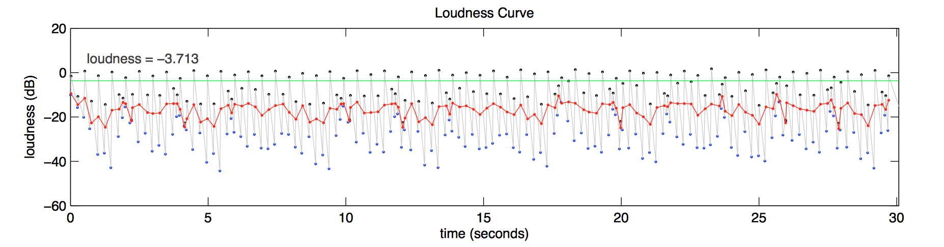
A Soundcloud April fools prank becomes reality.
A research paper by Karthik Yadati, Martha Larson, Cynthia C. S. Liem, Alan Hanjalic at Delft University of Technology (2014)
http://www.terasoft.com.tw/conf/ismir2014/proceedings/T026_297_Paper.pdf
The Soundcloud prank (2013)
http://www.attackmagazine.com/news/soundcloud-when-april-fools-day-pranks-go-wrong/
Analog spectrum analyzer by Albert Michelson circa. 1897
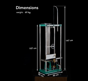
Documentary by Bill Hammack
Paper by Bill Hammack, Steve Kranz, and Bruce Carpenter
http://www.engineerguy.com/fourier/pdfs/albert-michelsons-harmonic-analyzer.pdf
What could it possibly have to do with my life?
-from X. Serra (2014) “Audio Signal Processing for Music Applications”
Humans are very good at pattern recognition. Is it a survival mechanism? People who listen to music are very good at analysis. Compared to the abilities of an average child, computer music information retrieval has not yet reached the computational ability of a worm: https://reactivemusic.net/?p=17744
(in computer science)
High-level
Low-level
(These demonstrations will be done in Ubuntu Linux 14.04.1)
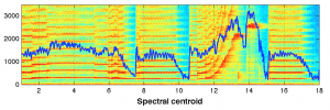
1a. Harmonic plus residual model (HPR) in sms-tools (speech-female 150-200 Hz. , and sax phrase)
1b. Do the same thing with transformation model
What about pitch salience and chroma?
(use workspace/A9)
import soundAnalysis as SA
Here is the list of descriptors that are donwloaded:
Index — Descriptor
16 — lowlevel.mfcc.mean.5
What happens when you look at multiple descriptors
In [22]: SA.descriptorPairScatterPlot( ‘tmp’, descInput=(0,5))
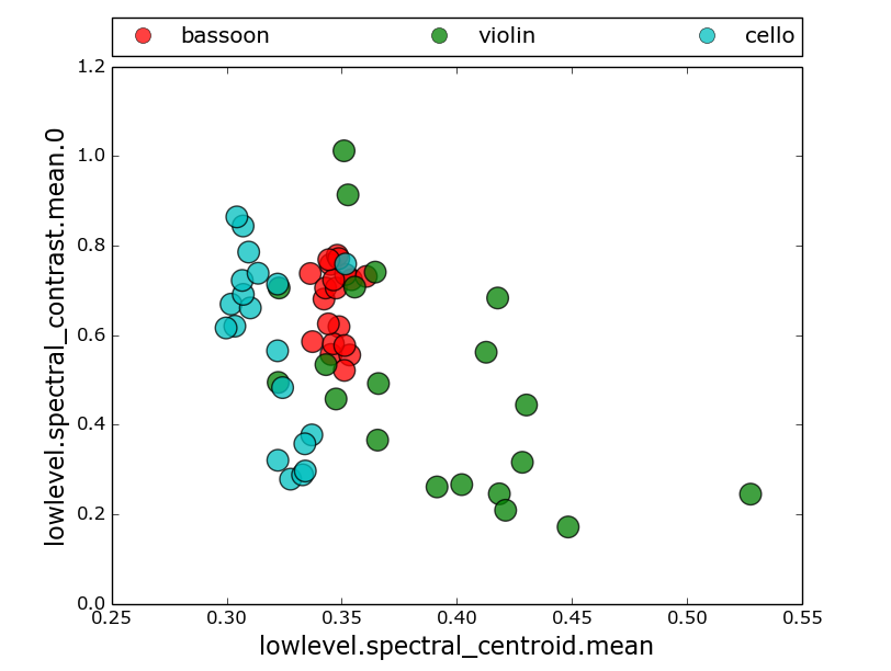
What descriptors best classify sounds into instrument groups?
SA.clusterSounds(‘tmp’, nCluster = 3, descInput=[0,2,9])
In [21]: SA.clusterSounds(‘tmp’, nCluster = 3, descInput=[0,2,9])
(Cluster: 0) Using majority voting as a criterion this cluster belongs to class: violin
Number of sounds in this cluster are: 15
sound-id, sound-class, classification decision
[[‘61926’ ‘violin’ ‘1’]
[‘61925’ ‘violin’ ‘1’]
[‘153607’ ‘violin’ ‘1’]
[‘153629’ ‘violin’ ‘1’]
[‘153609’ ‘violin’ ‘1’]
[‘153608’ ‘violin’ ‘1’]
[‘153628’ ‘violin’ ‘1’]
[‘153603’ ‘violin’ ‘1’]
[‘153602’ ‘violin’ ‘1’]
[‘153601’ ‘violin’ ‘1’]
[‘153600’ ‘violin’ ‘1’]
[‘153610’ ‘violin’ ‘1’]
[‘153606’ ‘violin’ ‘1’]
[‘153605’ ‘violin’ ‘1’]
[‘153604’ ‘violin’ ‘1’]]
(Cluster: 1) Using majority voting as a criterion this cluster belongs to class: bassoon
Number of sounds in this cluster are: 22
sound-id, sound-class, classification decision
[[‘154336’ ‘bassoon’ ‘1’]
[‘154337’ ‘bassoon’ ‘1’]
[‘154335’ ‘bassoon’ ‘1’]
[‘154352’ ‘bassoon’ ‘1’]
[‘154344’ ‘bassoon’ ‘1’]
[‘154338’ ‘bassoon’ ‘1’]
[‘154339’ ‘bassoon’ ‘1’]
[‘154343’ ‘bassoon’ ‘1’]
[‘154342’ ‘bassoon’ ‘1’]
[‘154341’ ‘bassoon’ ‘1’]
[‘154340’ ‘bassoon’ ‘1’]
[‘154347’ ‘bassoon’ ‘1’]
[‘154346’ ‘bassoon’ ‘1’]
[‘154345’ ‘bassoon’ ‘1’]
[‘154353’ ‘bassoon’ ‘1’]
[‘154350’ ‘bassoon’ ‘1’]
[‘154349’ ‘bassoon’ ‘1’]
[‘154348’ ‘bassoon’ ‘1’]
[‘154351’ ‘bassoon’ ‘1’]
[‘61927’ ‘violin’ ‘0’]
[‘61928’ ‘violin’ ‘0’]
[‘153769’ ‘cello’ ‘0’]]
(Cluster: 2) Using majority voting as a criterion this cluster belongs to class: cello
Number of sounds in this cluster are: 23
sound-id, sound-class, classification decision
[[‘154334’ ‘bassoon’ ‘0’]
[‘61929’ ‘violin’ ‘0’]
[‘61930’ ‘violin’ ‘0’]
[‘153626’ ‘violin’ ‘0’]
[‘42252’ ‘cello’ ‘1’]
[‘42250’ ‘cello’ ‘1’]
[‘42251’ ‘cello’ ‘1’]
[‘42256’ ‘cello’ ‘1’]
[‘42257’ ‘cello’ ‘1’]
[‘42254’ ‘cello’ ‘1’]
[‘42255’ ‘cello’ ‘1’]
[‘42249’ ‘cello’ ‘1’]
[‘42248’ ‘cello’ ‘1’]
[‘42247’ ‘cello’ ‘1’]
[‘42246’ ‘cello’ ‘1’]
[‘42239’ ‘cello’ ‘1’]
[‘42260’ ‘cello’ ‘1’]
[‘42241’ ‘cello’ ‘1’]
[‘42243’ ‘cello’ ‘1’]
[‘42242’ ‘cello’ ‘1’]
[‘42253’ ‘cello’ ‘1’]
[‘42244’ ‘cello’ ‘1’]
[‘42259’ ‘cello’ ‘1’]]
Out of 60 sounds, 7 sounds are incorrectly classified considering that one cluster should ideally contain sounds from only a single class
You obtain a classification (based on obtained clusters and majority voting) accuracy of 88.33 percentage
Which neighborhood or group does a sound belong to?
(using bad male vocal)
SA.classifySoundkNN(“qs/175454/175454/175454_2042115-lq.json”, “tmp”,13, descInput = [0,5,10])
===
from workspace…
First test: Use sounds by querying “saxophone”, tag=”alto-sax”
https://www.freesound.org/people/clruwe/sounds/119248/
I am using the same descriptors [0,2,9] that worked well in previous section. with K=3. Tried various values of K with this analysis and it always came out matching ‘violin’ which I think is correct.
In [26]: SA.classifySoundkNN(“qs/saxophone/119248/119248_2104336-lq.json”, “tmp”, 33, descInput = [0,2,9])
This sample belongs to class: violin
Out[26]: ‘violin’
Second test: I am trying out the freesound “similar sound” feature. Using one of the bassoon sounds I clicked “similar sounds” and chose a sound that was not a bassoon – “Bad Singer” (male).
http://freesound.org/people/sergeeo/sounds/175454/
Running the previous descriptors returned a match for violin. So I tried various other descriptors, and was able to get it to match bassoon consistently by using: [0,5,10] which are lowlevel.spectral_centroid.mean, lowlevel.spectral_contrast.mean.0, and lowlevel.mfcc.mean.0.
I honestly don’t know the best strategy for choosing these descriptors and tried to go with ones that seemed the least esoteric. The value of K does not seem to make any difference in the classification.
Here is the output
In [42]: SA.classifySoundkNN(“qs/175454/175454/175454_2042115-lq.json”, “tmp”,13, descInput = [0,5,10])
This sample belongs to class: bassoon
Out[42]: ‘bassoon’
#: cd ~/sms-tools/workspace/A9/qs/175454/175454
# cat 175454_2042115-lq.json | python -mjson.tool
(typical analysis page…) https://reactivemusic.net/?p=17641
fingerprinting and human factors like danceability…
random -> ordered (stochastic -> deterministic (for academics))
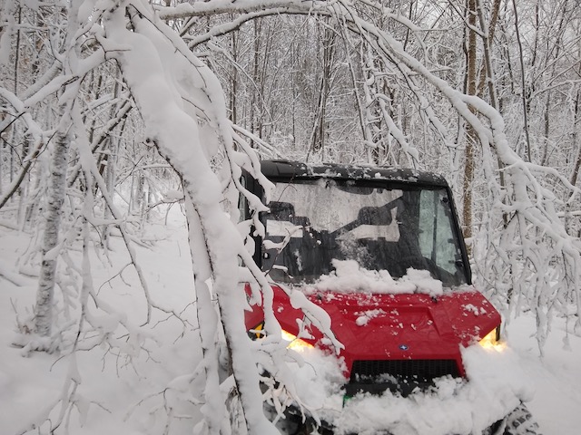
Does technology have a sound?
Brain wiring diagram: https://reactivemusic.net/?p=17758
Christof Koch – check out this video at around 13:33 for about 2 minutes http://www.technologyreview.com/emtech/14/video/watch/christof-koch-hacking-the-soul/
With every technology, musicians figure out how to use it another way. Starting with stone tools, bow and arrow, and now computers.
Data science skills: https://reactivemusic.net/?p=17707
At the end of the class we revved the engine of a 2015 Golf TSI, connected to an engine sound simulator in Max, on Boylston street…
https://reactivemusic.net/?p=7643
“Browse, download and share sounds”
By Frederic Font, Gerard Roma, and Xavier Serra. “Freesound technical demo.” Proceedings of the 21st ACM international conference on Multimedia. ACM, 2013.

Developer API: https://www.freesound.org/help/developers/
Low level features and timbre.
By Juan Pablo Bello at NYU
http://www.nyu.edu/classes/bello/MIR_files/timbre.pdf